To my main page
To my projects page
The applet at the bottom of this page simulates what happens over a transmission line both during sinusoidal steady state and when a transient signal is sent through the line.
Enter all of the parameters of the transmission line system. The source information includes the amplitude (A) and the phase offset in degrees (P) of the voltage source (Vg) as well as the real (R) and imaginary (I) components of the input source impedance (Zg). The geometric information that you have to enter includes the angular frequency (w) of the voltage source and the length (L) of the transmission line. Please note that as a reference in space, the load is located at point 0 and the source is located at point -L. The voltage source produces an output Vg(t)=Acos(wt+P).
The main voltage source that will be used in the calculations is the one that has its values in all of the text areas. You can, however, have additional single phase voltage sources connected in series. To have several voltage sources, just set their values (A,w, and P) and press the add button. Once you have the secondary sources, place the values of the main source and continue entering the rest of the values. The resulting voltage input will then be a summation of all of the separate (the main one and all of the secondary) voltage sources.
When multiple voltage sources are used then the input source impedance (Zg) becomes a resistor in series with either a capacitor or an inductor. When the imaginary component (I) of Zg is positive, then Zg is a resistor of value Real(Zg) in series with an inductor of value (The angular velocity of the single phase voltage source being examined)*Imaginary(Zg)/(The angular velocity of the main voltage source). When the imaginary component (I) of Zg is negative, then Zg is a resistor of value Real(Zg) in series with a capacitor of value 1/[(The angular velocity of the single phase voltage source being examined)*Imaginary(Zg)/(The angular velocity of the main voltage source)]. The same holds true for the load impedance. The diagram below shows the model of the transmission line that I am using.
After you have entered the source and geometric information please enter the transmission line information. You can either enter the real (R) and imaginary (I) components of gamma (G) and the real (R) and imaginary (I) components of the characteristic impedance (Zo) of the transmission line and then press the "Go Down" button to calculate the remaining values. Alternatively you can enter the resistance per unit length (R), the inductance per unit length (L), the conductance per unit length (G), and the capacitance of unit length (C) of the transmission line, and then press the "Go Up" button to calculate gamma and Zo. The real part of gamma represents the attenuation of the transmission line and the imaginary part represents the phase constant of the transmitted wave. Please note that for the calculations to occur all of the transmission line information must be consistent. That is gamma and Zo must correspond to the values of R, L, G, and C for the specified main voltage source. All of the secondary single phase voltage sources (if any) recalculate their own copies of gamma and Zo from the specified R, L, G, and C values.
The final piece of information that you have to give is the load impedance (Zl) including both its real (R) and imaginary (I) components. You can press the "Use Smith Chart" button to see a Smith chart which you can use to select the appropriate load impedance. The green dot represents the point on the Smith chart where the load impedance is in respect to the input impedance. The reflection coefficient (RC) and the Zo to Zl ratio (Z) as well as wavelengths towards load (WTL) and wavelengths towards generator (WTG) are given in the top left corner. The bottom left corner has the values for RC, Z, WTL, and WTG of the position where the mouse is currently located (if the mouse is within the circle of the Smith chart). To select a new Zl just press the left mouse button when the mouse is over the location on the graph where you want the load impedance to be. The green dot moves there and the information in the top left corner is updated. If you are satisfied with your selection press the "OK" button and Zl will be updated in the applet. To cancel your selection press the "Cancel" button.
Finally, if you put a check in the check box at the bottom left of the applet, then a transient analysis will be performed. If there is no check box there, then a sinusoidal steady state analysis will be performed. The parameter to the right of the check box is the speed factor (SF). This controls the time increment used for calculations. This can be used to slow down or speed at which the graphs will move. If transient analysis is performed, the speed factor can also determine if the system is stable or unstable. If the speed factor is too high, then the numerical analysis cannot converge and the graphs do not relay any useful information. Since the transient analysis is much slower than the steady state case, you should try to have a speed factor of 4 or 5 at first, and if the system is too unstable for you, you should decrease the factor.
Once you have entered all of the settings that you want, press the "Re-Calculate" button in the top right corner of the applet. Everything will be recalculated, you will see the proper values for the reflection coefficient (RC), the lossless voltage standing wave ratio (S), the wavelength (l), the phase velocity (u) and the current time (t) which corresponds to the graphs being displayed (at the beginning the time will be 0). After everything is recalculated you can press the play, stop, and pause buttons to view the graphs as time progresses. Play increments the time and updates the graphs. Stop causes the time to reset to 0 and not move. Pause causes the time to stop moving. The magnitude button works only when steady state analysis is performed and it shows the maximum amplitude of any sinusoidal wave passing through each point on the line (the button causes the time to stop moving as well). You can enter new information and recalculate as much as you want. The graphs that you see are the voltage, current, and the ratio of voltage to current at any specified point in space at some specific time that is equal to the current time (t) in the top right corner of the applet.
Please note that all of the values that you enter should be numbers and that the applet does not generally check to make sure that some of the numbers which should not be negative are in reality non-negative. Alse please note that in the transient analysis certain source impedance and load impedance values can cause the system to become unstable. These occur when the load resistance is really small (or 0) and the resistance is in series with a capacitance. This is especially troublesome when the reflection coefficient has a magnitude of almost 1 and a degree of somewhere between -115 and -180 degrees. The system can also be unstable if the source impedance is a large resistor in series with an inductor. Both of these situations are unstable because they lead to multiplicative factors (at the load the equation has a 1/R factor and at the source the equation has an R factor) in the numerical approximations that are too large and therefore lead to instability. I would have included this information as part of the applet explanation, but since this is a limiting factor for the input I decided to give this explanation here.
Also please note that for the transient analysis I make the voltage sources output their values for one period of the main voltage source. Outside of that time the voltage sources act as a short circuit. Since the numerical analysis does not like sudden changes in voltage, if you want the system to be stable you should ensure that at time 0, the superposition of all the voltage sources is equal to 0. Actually, real life doesn't like instantaneous change either. If the voltage at a capacitor changed instantly, infinite current would be produced (i=C dv/dt), and that is impossible. Also, if the transient analysis is unstable, just lower the speed factor. The lower the speed factor, the more stable the analysis becomes; although it does also take longer.
The applet uses the standard telegraphers equations and phasor analysis to calculate the sinusoidal steady state response. The applet also uses numerical approximations of the tepegraphers equations as well as of the basic linear circuits that contain resistors, capacitors, and inductors to calculate the transient response of the system.
The steady state analysis tries to identify v(z,t) and i(z,t) for all points and all time. The following defines the steps needed to solve for v(z,t) and i(z,t) in the sinusoidal steady state. In the sinusoidal steady state v and i can be represented in phasor form as v(z,t)=Re{V(z)exp(jwt)} and i(z,t)=Re{I(z)exp(jwt), where w is the angular frequency of the sinusoid. The telegraphers equations, which can be derived by looking at a small seciton of a transmission line, then become d^2V(z)/dz^2 - G^2V(z)=0 and d^2I(z)/dz^2 - G^2I(z)=0 where V(z) and I(z) are the phasors, G is gamma which is equal to sqrt((R'+jwL')(G'+jwC')) where R' is the resistance per unit length, L' the inductance per unit length, G' the conductance per unit length, and C' the capacitance of unit length of the transmission line. The characteristic impedance (Zo) of the transmission line is equal to sqrt((R'+jwL')/(G'+jwC')). To go from G and Zo to R', L', G', and C' I used the equations GZo=R'+jwL' and G/Zo=G'+jwC'.
V(z) is the sum of a wave moving to the right (with a voltage of Voplus*exp(-Gz) and a current of Ioplus*exp(-Gz)) and a wave moving to the left (with a voltage of Vominus*exp(Gz) and a current of Iominus*exp(Gz)). The reflection coefficient (RC) can then be defined as: RC = Voplus/Vominus = (Zl-Zo)/(Zl+Zo) where Zl is the load impedance. Please note that Zo = Voplus/Ioplus = -Vominus/Iominus. V(z) and I(z) can then be rewritten as [exp(-Gz)+RCexp(Gz)]Voplus and [exp(-Gz)-RCexp(Gz)]Voplus/Zo respectively. The phase velocity (u) is defined as w/Im{G}, the wavelength, lambda (l) is defined as 2PI/Im{G}, and the voltage standing wave ratio (S) is defined as (1+|RC|)/(1-|RC|).
The input impedance as looking in from the left to the right at
point z is: Zin(z) = V(z)/I(z) = Zo[(1+RCexp(2Gz))/(1-RCexp(2Gz))]
When the voltage source is located at location -L with a phasor
voltage of Vg and an impedance of Zg then the voltage on the
transmission line at point -L is:
V(-L) = Voplus[exp(GL)-RCexp(-GL)] = Vg*Zin(-L)/(Zg+Zin(-L)).
Solving for Voplus yields:
Voplus = (Vg*Zin(-L)/(Zg+Zin(-L))/(exp(GL)-RCexp(-GL))
After all of this, Voplus, Zo, G, and RC are known. V(z) and I(z) are therefore known and so v(z,t) and i(z,t) can be calculated for all values of z and t. The preceding are all of the steps required for the sinusoidal steady state analysis. The time increment between frames for the steady state graphs is 0.05*(Speed Factor)/w.
The transient analysis uses a different form of the telegrapher's
equations. The two equations that the analysis uses are
-dv(z,t)/dz=R'i(z,t)+L'di(z,t)/dt and
-di(z,t)/dz=G'v(z,t)+L'dv(z,t)/dt. Turning these into numerical approximations
where a forward differential equation is used for the derivative in time
and a centre weighted approximation is used for the derivative in space the
result is:
i(z,t+dt)=i(z,t)-[R'i(z,t)+(v(z+dz,t)-v(z-dz,t))/2dz]*dt/L'
v(z,t+dt)=v(z,t)-[G'v(z,t)+(i(z+dz,t)-i(z-dz,t))/2dz]*dt/C'
These, however, are still equations with continues variables. I only care about the values of these equations at certain points. To do that I have defined 1/2dz as the number of data points in my array divided by the length of the transmission line and I have defined dt as 0.001*(Speed factor)*Im{G}/w, which is equal to 0.001*(the phase velocity of the wave)*(Speed factor), although each frame that is shown in the transient analysis represents an increment of 500dt. Please note that I will represent the number of data points in my array is either points, or just p.
I defined the points in my arrays as V[t][k]=v(-L+1.5dz+2kdz,t) and I[t][k]=(-l+0.5dz+2kdz,t). This definition allows me to place the voltage points and current points a little bit apart (dz) away from each other. The reason why I can do that is that the centre weighted approximation of the space derivative does not actually depend on the value at the centre, just at the two points to the left and to the right. My array values go from 0 to points-1. The way I have set up the array means that i(z,t), v(z+dz,t), and v(z-dz,t) become I[t][k], V[t][k], and V[t][k-1] respectively and that v(z,t), i(z+dz,t), and i(z-dz,t) become V[t][k], I[t][k+1], and I[t][k] respectively. Of course there is a problem when k=0 or when k=points-1. Then I need to know V[t][-1] and I[t][points], which are just outside of the transmission line, at the boundaries. To do this, I use the equations for circuits that just contain resistors, capacitors, and inductors (more on this a little later). The way I have combined the two arrays is shown in the figure below.
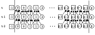
Please note that the square boxes represent the voltage, that the circles represent the current, and that the arrows show the direction of propagation for the various values (for example I[t][0] is derived from V[t-1][-1], I[t-1][0], and V[t-1][0] while V[t][0] is derived from I[t-1][0], V[t-1][0], and I[t-1][1]). The time index is shown on the left, although it is arbitrary. The two vertical lines represent the boundaries of the transmission line. The distance between each square and circle is dz. I[t][0] is located 0.5dz to the right of the left boundary of the transmission line while V[t][p-1] is located 0.5dz to the left of the right boundary of the transmission line.
The equations that I use at the left boundary (where the voltage source is located) are V[t][-1]=V[t-1][-1]+Vg[t]-Vg[t-1]+Rg(I[t-1][0]-I[t][0])-I[t][0]dt/Cg if I have a capacitor and a resistor in series (even if the resistor has a resistance of 0) and v[t][-1]=Vg[t]-I[t]Rg-(I[t][0]-I[t-1][0])Lg/dt if I have a resistor in series with an inductor (even if one of them or both of them have a value of 0). Here Vg is the input source voltage (which can be several voltage sources in series), Rg is the input resistance, Lg is the input inductance, and Cg is the input capacitance. As stated beforehand if Rg or Lg become too large, the system becomes unstable. It can be seen why this would be the case from the previous equations. Also, if Cg were to be made really small, the system would become unstable as well.
In the preceding Rl is the load resistance, Cl is the load capacitance, and Ll is the load inductance. Please note that in the above equations there are many places where the system is unstable. For example when there is a short circuit, in reality i[t][p]=v[t][p-1]/0, but this is undefined. So I tried replacing it with a small section of the transmission line that is short circuited at the right end. Although this does not give the proper result, the results phase is off by only about 10 degrees. Also whenever Rl is really small any equation with 1/Rl can be a problem. The same goes for Ll and Cl. For some equations if Rl or Cl are too large, problems can arise as well. So please watch out, and if you do need to use values which cause the equation to be unstable, then please decrease the speed factor accordingly. Although the short circuit case will probably not work properly anyway.
The default options just cause the wave to travel as if the line were infinite (there's no reflection). For interesting effects you should turn transient analysis on, set L in the geometric information as 10 (so as to see the single wave travel), and P in source information to -90 (this is the phase of the cosine and this is necessary because finite differential solutions cannot cope with discontinuities). Press re-calculate and then see the wave go and get reflected.
Finally, after all that text, here's the applet.
This web page is maintained by Borys
Bradel. Last update: Sep. 24, 2001
Address:
http://www.eecg.utoronto.ca/~bradel/projects/transmissionline/index.html